Introduction

This blog post ommits some citations due to visualisation purposes, for a full list of references please refer to the whitepaper version which was written for a seminar during my graduate studies. There is also a presentation available.

With recent advances in machine learning the size of training data and the size of deep neural network models is heavily increasing which raises demand for better performing optimization algorithms. Common approaches are either improving the computational steps of the optimization algorithms or introducing parallel computing to speed up convergence. Using a fixed mini-batch size for each process in parallel computing causes the mini-batch size of the overall system to linearly scale with the number of processes. As the mini-batch size increases past a threshold the validation accuracy decreases. Other works tried to overcome this by varying the learning rate and batch size over epochs. Now, ¹ tries to tackle this large mini-batch problem with taking a more mathematically rigorous approach where they assume that large mini-batches become more statistically stable which introduces advantages for second-order optimization methods. In this blog post I want to summarize the main contribution while also giving a little more background information on some parts to get a better understanding of the topic.

Notation

In our notation the training data \(\mathcal{T}=\left\{\left(\mathbf{x}_{1}, \mathbf{y}_{1}\right),\left(\mathbf{x}_{2}, \mathbf{y}_{2}\right), \cdots,\left(\mathbf{x}_{n}, \mathbf{y}_{n}\right)\right\}\) consists of \(n\) feature-label pairs. Here, each \(\mathbf{x}_{i} \in \mathbb{R}^{d_{x}}\) is the feature vector and \(\mathbf{y}_{i} \in \mathbb{R}^{d_{y}}\) is the label vector with their respective sizes \(d_{x}\) and \(d_{y}\). The deep learning model is described as a mapping \(F(\cdot ; \boldsymbol{\theta}): \mathcal{X} \rightarrow \mathcal{Y}\) from the feature space \(\mathcal{X}\) to the label space \(\mathcal{Y}\) where \(\boldsymbol{\theta}\) are the parameters of the model. This leaves us with a model notation which when presented with an input instance \(\mathbf{x}_{i} \in \mathcal{X}\) yields a predicted output denoted as \(\hat{\mathbf{y}}_{i}=F\left(\mathbf{x}_{i} ; \boldsymbol{\theta}\right)\). The difference of the true label \(\mathbf{y}_{i} \in \mathcal{Y}\) to this predicted label \(\hat{\mathbf{y}}_{i}\) is then described as the loss term \(\ell\left(\hat{\mathbf{y}}_{i}, \mathbf{y}_{i}\right)\) which can have different definitions based on the specific problem (e.g. Mean Squared Error, Hinge Loss, Cross Entropy Loss, etc.). By summing up over all data points in the training data we get the total loss term defined as:

\[\mathcal{L}(\boldsymbol{\theta} ; \mathcal{T})=\sum_{\left(\mathbf{x}_{i}, \mathbf{y}_{i}\right) \in \mathcal{T}} \ell\left(\hat{\mathbf{y}}_{i}, \mathbf{y}_{i}\right)\]

During training we try to optimize the model parameters \(\boldsymbol{\theta} \in \mathbb{R}^{d_{\theta}}\), which are part of the variable domain \(\Theta\), by minimizing the total loss on the training set. This can be described as:

\[\min _{\boldsymbol{\theta} \in \Theta} \mathcal{L}(\boldsymbol{\theta} ; \mathcal{T})\]

For this process of finding a global or local minimum for convex and non-convex loss surfaces, a variety of different optimization algorithms are available. Most of these algorithms use the learning rate \(\eta\) to determine the step sizes taken for the parameters \(\boldsymbol{\theta}\) at each update step \(\tau\) in the opposite direction of the gradient of the loss function \(\nabla_{\boldsymbol{\theta}} \mathcal{L}(\boldsymbol{\theta}^{(\tau-1)} ; \cdot)\). Here, \(\boldsymbol{\theta}^{(\tau)}\) are the parameters of the model at the update step \(\tau\) with \(\tau \geq 1\). The initialized hyperparameter values are denoted as \(\boldsymbol{\theta}^{(0)}\).

Related Work

Related Work in the realm of Deep Learning Optimizers can broadly be classified in First- and Second-Order Optimization Algorithms. Here we want to give a quick overview over those two areas.

First-Order Optimization Algorithms

There are various First-Order Optimization Algorithms which are widely used in Deep Learning. One of the most popular choices due to its simplicity is still Stochastic Gradient Descent (SGD) with the update rule:

\[\boldsymbol{\theta}^{(\tau)}=\boldsymbol{\theta}^{(\tau-1)}-\eta \cdot \nabla_{\boldsymbol{\theta}} \mathcal{L}\left(\boldsymbol{\theta}^{(\tau-1)} ;\left(\mathbf{x}_{i}, \mathbf{y}_{i}\right)\right)\]

However, there have been recent advances yielding new and improved First-Order Optimizers such as Adam, AdamW, AMSGrad, AdaBound, AMSBound, RAdam, LookAhead, Ranger and many more which offer time-convergence improvements based on Adaptive Gradient methods and Momentum Terms.

Second-Order Optimization Algorithms

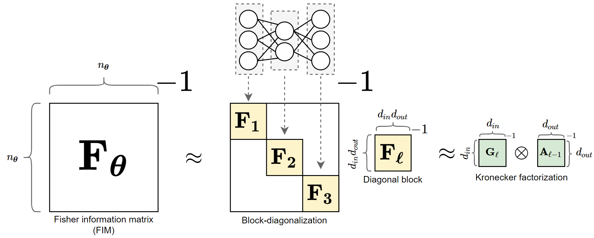
The generalized Gauss-Newton-Method and Natural Gradient Descent (NGD) set the groundwork for improvements on Second-Order Optimization Algorithms. Such work yielded the Kronecker-factored Approximate Curvature (K-FAC) which effeciently approximates the empirical Fisher information matrix (FIM) \(\mathbf{F}_{\boldsymbol{\theta}}\) given in the next Equation through block-diagonalization and Kronecker factorization of these blocks:

\[\mathbf{F}_{\boldsymbol{\theta}} = \mathop{\mathbb{E}}_{p(\mathbf{x},\mathbf{y})}\left[\nabla \log p(\mathbf{y}|\mathbf{x};\boldsymbol{\theta}) \nabla \log p(\mathbf{y}|\mathbf{x};\boldsymbol{\theta})^T\right]\]

For a neural network with \(L\) Layers K-FAC approximates \(\mathbf{F}_{\boldsymbol{\theta}}\) as displayed in the next Equation with \(\mathbf{F}_\ell\) being the block matrix for the FIM of the \(\ell\) th layer:

\[\mathbf{F}_{\boldsymbol{\theta}} \approx \operatorname{diag}\left(\mathbf{F}_1, \mathbf{F}_2, \dots, \mathbf{F}_\ell, \dots \mathbf{F}_L \right)\]

Each block is then approximated using the Kronecker-factorization:

\[\mathbf{F}_\ell \approx \mathbf{G}_\ell \otimes \mathbf{A}_{\ell-1}\]

With the properties of the Kronecker-factorization we can write the blocks as:

\[\mathcal{G}_\ell^{(\tau-1)} = \left({\mathbf{G}_\ell^{(\tau-1)}}^{-1} \otimes {\mathbf{A}_{\ell-1}^{(\tau-1)}}^{-1}\right)\]

Now using the NGD update rule we get the update rule for the parameters \(\boldsymbol{\theta}_\ell^{(\tau)}\):

\[\boldsymbol{\theta}_\ell^{(\tau)} = \boldsymbol{\theta}_\ell^{(\tau-1)} - \eta \cdot \mathcal{G}_\ell^{(\tau-1)} \cdot \nabla \mathcal{L}_\ell\left(\boldsymbol{\theta}_\ell^{(\tau-1)};\cdot\right)\]

To get a more intuitive and visual approach to the FIM approximation as well as the Kronecker-product lets look at some visualisations. Figure 1 shows the Approximation of the FIM used in K-FAC. This shows that the FIM gets block-diagonalized with \(\mathbf{F}_\ell\) being the block matrix for the FIM of layer \(\ell\). In particular, the FIM of each layer consists of the weights for that specific layer. Each block gets then further approximated using the Kronecker-factorization.

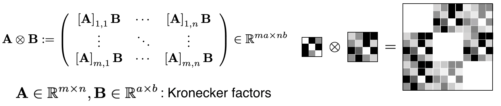
The Kronecker-factorization is visually shown in figure 2 (taken from ²). When we assume a white space corresponds to \(0\), a black space corresponds to \(1\) and a grey space corresponds to any other value between \(0\) and \(1\) the resulting matrix has the shape of multiplying the dimenstions of the two Kronecker-factors. This can basically be thought of as arranging the product of matrix \(\mathbf{B}\) with each cell of matrix \(\mathbf{A}\) in a new matrix. Because matrix \(\mathbf{A}\) has white diagonal elements the resulting matrix also has white block-diagonal elements. Black elements in matrix \(\mathbf{A}\) result in matrix \(\mathbf{B}\) being put in that position while grey elements yield new alternated entries.

If we now take a look at the approximation process for AlexNet in figure 3 which is a common architecture for image classification we can see the degree of computational improvement this approach offers. AlexNet has \(60,000,000\) parameters which yields a Fisher information matrix with shape \(\mathbf{F}_{\boldsymbol{\theta}} \in \mathbb{R}^{60,000,000 \times 60,000,000}\) which needs to be inverted in order to make one iteration in updating the parameters when using the NGD update rule. If we now take a look at the last block-approximated diagonal block which corresponds to the last AlexNet layer, we observe that it has the shape \(\mathbf{F}_\ell \in \mathbb{R}^{4,096,000 \times 4,096,000}\) which can further be approximated by two smaller matrices where \(\mathbf{A}_{\ell - 1} \in \mathbb{R}^{4,096 \times 4,096}\) is the input to layer \(\ell\) and \(\mathbf{G}_\ell \in \mathbb{R}^{1,000 \times 1,000}\) is the output of layer \(\ell\). The fact that we don't need to invert those enormous matrices but these rather small matrices show how much computational improvement this approach actually offers. Using this approximation for the FIM is the main property which distinguishes K-FAC from NGD and without it K-FAC wouldn't perform much different from regular NGD.

Besides the problem of inverting infeasible large matrices such as the FIM or the Hessian, which K-FAC tries to solve, a common drawback for Second-order optimizers is the complexity to optimize them for distributed computing. This is where Osawa et al. try to contribute a method which will improve the state-of-the-art.

Parallelized K-FAC

The design which gets proposed by Osawa et al. is visualised in figure 4.

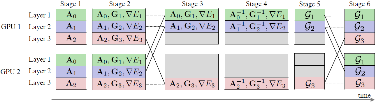
Each stage corresponds to a needed step of computation, here representative with \(2\) GPUs and a \(3\) layer neural network. In the first two stages \(\mathbf{A_{\ell-1}}\) and \(\mathbf{G}_\ell\) get computed by forward and backward passing the input through the network. For that, each process uses different mini-batches to calculate the Kronecker factors. After that, the values of these factors get summed up to calculate the global factors and the results get distributed to the different processes (ReduceScatterV) to keep model-parallelism. The purpose of distributing the results to each process is so that every GPU can compute the preconditioned gradient \(\mathcal{G}_\ell\) for a different layer \(\ell\). If there are more layers than processes then one process computes multiple preconditioned gradients as shown in Stage \(3\) of figure 4. Stage \(4\) and Stage \(5\) are respectively the inverse computation stage and the matrix multiplication stage. After stage \(5\) we distribute each \(\mathcal{G}_\ell\) to each process (AllGatherV) to reach stage \(6\) where each process can now update the parameters \(\boldsymbol{\theta}\) by using the preconditioned gradients. Osawa et al. also use some methods to speed up communication, use damping for the FIM to make training more stable as well as learning rate schedules and momentum for K-FAC to speed up convergence. These methods are not explicitly explained here since they are not the main contribution of this work and have been applied in other settings as well.

Results

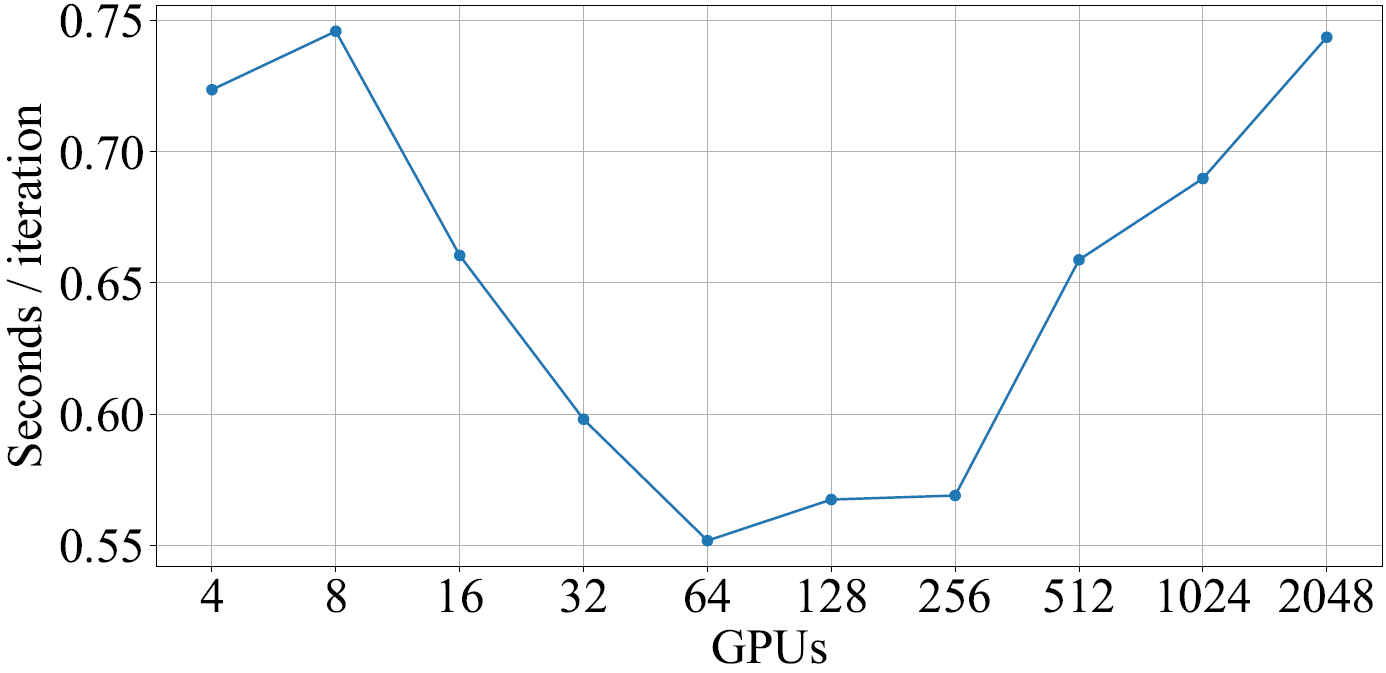
Their results show that the optimal amount of GPUs to use for their experimental setup is \(64\). After that, the overhead for communication becomes too large which causes a sharp increase in iteration cost.

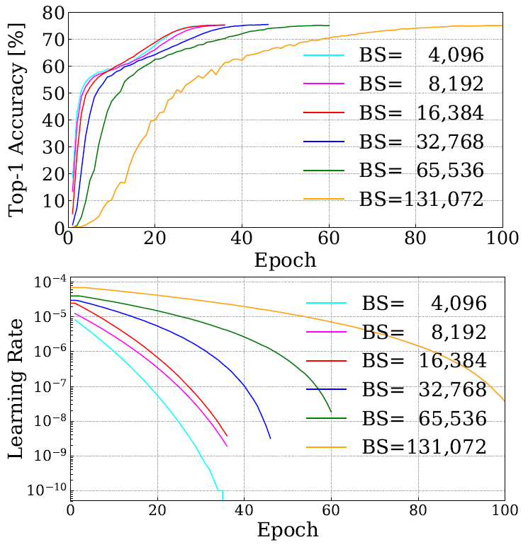
They are able to achieve a really competitive validation accuracy of $\geq 75\%$ using really large batch sizes (BS) which none other first-order optimization method is able to sustain. The respective training curves with their learning rates and batch sizes are shown in figure 6. If we compare the batch sizes for other first-order based methods on the same problem set we can see that the high validation accuracies (\(\sim76\%\)) achieved by those methods commonly use batch sizes \(\leq 32\text{K}\).

Conclusion & Outlook

Generally, with the obtained results Osawa et al. were able to show that parallelized second-order optimization algorithms do in fact generalize relatively similar to SGD approaches even for large mini-batch sizes. This is a result which is new in its entirety since first-order methods are thought of as having a large edge over second-order alternatives. However, their approach can still be improved by improving the communication complexity as well as approximating the Kronecker-factors without loss of accuracy. For further improvements they mention that each speed-up method for SGD which they applied to their approach improved convergence similar to the effect it has on SGD. This property opens up the field for further improvements on second-order optimization algorithms by the possibility of further applying already known speed-up techniques for first-order methods.